Python Fundamentals III: data analysis
This interactive lesson will focus on two of the foundational python libraries for data analysis (numpy and pandas), for working with numerical data and heterogeneous tabular data.
1. NumPy: what and why
NumPy (Numerical Python) is an open source Python library that’s widely used in science and engineering. The NumPy library contains multidimensional array data structures.
It can be imported as follows:
import numpy as np
[1]:
import numpy as np
1.1 What is an array?
Here is an example of a one-dimensional (1x4) array with int data:
\(\begin{array}{|c|c|} \hline 1 & 5 & 2 & 0 \\ \hline \end{array}\)
A two-dimensional array would be a table (example: 3x4 array):
\(\begin{array}{|c|c|} \hline 1 & 5 & 2 & 0 \\ \hline 8 & 3 & 6 & 1 \\ \hline 1 & 7 & 2 & 9 \\ \hline \end{array}\)
A three-dimensional array would be a “cube”, or a stack of tables, and so on.
Let’s see how to create arrays in numpy!
[2]:
# 1D array: simply create a list of numbers and use np.array(...)

a = np.array([1,5,2,0])
a
[2]:
array([1, 5, 2, 0])
[3]:
# 2D array: create a list of lists of numbers!
# All inner lists must have the same length to make a "squared" table.
# Then use  np.array(...) to transform it into an actual array.

b = np.array(
    [
        [1,5,2,0],
        [8,3,6,1],
        [1,7,2,9]
    ]
)
b
[3]:
array([[1, 5, 2, 0],
       [8, 3, 6, 1],
       [1, 7, 2, 9]])
[4]:
# 3D array: any guesses?

c = np.array(
    [
        [
            [1,5,2,0],
            [8,3,6,1],
            [1,7,2,9]
        ],
        [
            [0,1,4,0],
            [7,3,9,1],
            [8,2,4,8]
        ],
    ]
)
c
[4]:
array([[[1, 5, 2, 0],
        [8, 3, 6, 1],
        [1, 7, 2, 9]],

       [[0, 1, 4, 0],
        [7, 3, 9, 1],
        [8, 2, 4, 8]]])
1.2 Why not lists?
Python lists are excellent, general-purpose containers. They can be “heterogeneous”, meaning that they can contain elements of a variety of types.
NumPy shines when there are large quantities of “homogeneous” (same-type) data to be processed on the CPU. They can improve speed, reduce memory consumption, and offer a high-level syntax for performing a variety of common processing tasks.
1.3 Getting information from the arrays
Usually, the things you are interested in knowing from an array are the following:
shape (how many rows, columns, etc) example:
b.shapenumber of dimensions example:
len(b.shape)orb.ndimnumber of elements in the array (if you don’t want to calculate it manually by multiplying the shape) example:
b.sizetype of elements in the array example:
b.dtype(data type) these could be int64 (integer, 64 bit), float64 (floating point number, 64 bit), bool (boolean values) or many more
[5]:
print(b)

print("-"*20)

print(f"Shape of the array: {b.shape}")
print(f"Number of dimensions: {len(b.shape)}")
print(f"How many elements: {b.size}")
print(f"Type of the elements: {b.dtype}")
[[1 5 2 0]
 [8 3 6 1]
 [1 7 2 9]]
--------------------
Shape of the array: (3, 4)
Number of dimensions: 2
How many elements: 12
Type of the elements: int64
[6]:
# you can change the type of the array!
# let's see some more dtypes

b_float = b.astype(float)
print(b_float)
print(f"Type of the elements: {b_float.dtype}")

print("-"*50)

b_bool = b.astype(bool)
print(b_bool)
print(f"Type of the elements: {b_bool.dtype}")

print("-"*50)

b_smallint = b.astype("int8")
print(b_smallint)
print(f"Type of the elements: {b_smallint.dtype}")
[[1. 5. 2. 0.]
 [8. 3. 6. 1.]
 [1. 7. 2. 9.]]
Type of the elements: float64
--------------------------------------------------
[[ True  True  True False]
 [ True  True  True  True]
 [ True  True  True  True]]
Type of the elements: bool
--------------------------------------------------
[[1 5 2 0]
 [8 3 6 1]
 [1 7 2 9]]
Type of the elements: int8
1.4 Accessing arrays
Here we will see ways to select elements with increasing freedom!
(1/3) Basic indexing (elements and rows/columns)
a[0]: get element in position 0b[1,2]orb[1][2]: get element in row 1, column 2c[1,0,2]orc[1][0][2]: get element at index 1 in the first dimension, index 0 in the second dimension, index 2 in the third dimension
In high-dimensional arrays, you can access full rows/columns/sub-arrays (instead of just an element) by leaving out some indices. The indices you “leave out” can be replaced with “:” or completely skipped (if they are the last index)
b[0,:]orb[0]: get row 0 of the matrix bb[:,0]: get column 0 of the matrix b
[7]:
# ACCESSING ELEMENTS

# 1D array

print("--- Vector a ---")
print(a)
print("\n--- Vector a, element 0 ---")
print(a[0])
print("\n--- Vector a, element 1 ---")
print(a[1])

# 2D array

print("\n\n--- Matrix b ---")
print(b)
print("\n--- Matrix b, element in row 1, column 2 ---")
print(b[1,2])
print(b[1][2])

# 3D array

print("\n\n--- Matrix c ---")
print(c)
print("\n--- Matrix c, element in position 1, 0, 2 ---")
print(c[1,0,2])
print(c[1][0][2])
--- Vector a ---
[1 5 2 0]

--- Vector a, element 0 ---
1

--- Vector a, element 1 ---
5


--- Matrix b ---
[[1 5 2 0]
 [8 3 6 1]
 [1 7 2 9]]

--- Matrix b, element in row 1, column 2 ---
6
6


--- Matrix c ---
[[[1 5 2 0]
  [8 3 6 1]
  [1 7 2 9]]

 [[0 1 4 0]
  [7 3 9 1]
  [8 2 4 8]]]

--- Matrix c, element in position 1, 0, 2 ---
4
4
[8]:
# ACCESSING ROWS/COLUMNS

print("--- Matrix b ---")
print(b)

print("\n\n--- Matrix b, row 0 ---")
print(b[0])
print(b[0,:])
print(b[0][:])

print("\n\n--- Matrix b, column 0 ---")
print(b[:,0])
--- Matrix b ---
[[1 5 2 0]
 [8 3 6 1]
 [1 7 2 9]]


--- Matrix b, row 0 ---
[1 5 2 0]
[1 5 2 0]
[1 5 2 0]


--- Matrix b, column 0 ---
[1 8 1]
(2/3) Advanced slicing
Like with lists, you can select slices of the arrays
b[0, 0:2]get in row 0, and select the elements from column 0 to column 2 (excluded)c[0, 0:2, :]get in position 0 of the first dimension, and select the elements from 0 to 2 (excluded) in the second dimension, and keep all in the third dimension.
b[0, [0,2]]get in row 0, and select the elements from column 0 and 2c[0, [0,2], :]get in position 0 of the first dimension, and select the elements at index 0 and 2 in the second dimension, and keep all in the third dimension.
[9]:
# ACCESSING SLICES

print("--- Matrix b ---")
print(b)

print("\n--- Matrix b, row 0, columns from 0th to 2nd (excluded) ---")
print(b[0, 0:2])


print("\n\n--- Matrix c ---")
print(c)

print("\n--- Matrix c, row 0, 'columns' from 0th to 2nd (excluded) ---")
print(c[0, 0:2, :])
--- Matrix b ---
[[1 5 2 0]
 [8 3 6 1]
 [1 7 2 9]]

--- Matrix b, row 0, columns from 0th to 2nd (excluded) ---
[1 5]


--- Matrix c ---
[[[1 5 2 0]
  [8 3 6 1]
  [1 7 2 9]]

 [[0 1 4 0]
  [7 3 9 1]
  [8 2 4 8]]]

--- Matrix c, row 0, 'columns' from 0th to 2nd (excluded) ---
[[1 5 2 0]
 [8 3 6 1]]
[10]:
# ACCESSING NON-CONTIGUOUS INDICES

print("--- Matrix b ---")
print(b)

print("\n--- Matrix b, row 0, columns 0 AND 2 ---")
print(b[0, [0,2]])

print("\n\n--- Matrix c ---")
print(c)

print("\n--- Matrix c, row 0, 'columns' 0 AND 2 ---")
print(c[0, [0,2]])
--- Matrix b ---
[[1 5 2 0]
 [8 3 6 1]
 [1 7 2 9]]

--- Matrix b, row 0, columns 0 AND 2 ---
[1 2]


--- Matrix c ---
[[[1 5 2 0]
  [8 3 6 1]
  [1 7 2 9]]

 [[0 1 4 0]
  [7 3 9 1]
  [8 2 4 8]]]

--- Matrix c, row 0, 'columns' 0 AND 2 ---
[[1 5 2 0]
 [1 7 2 9]]
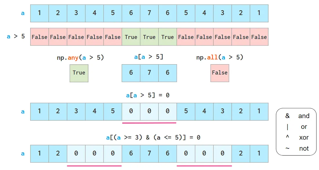
(3/3) Anything, anywhere: Boolean Masks
Another super-useful way of getting data from NumPy arrays is boolean indexing, which allows using all kinds of logical operators.
[11]:
print("--- Matrix b ---")
print(b)

# Create a boolean mask
mask = b > 5
print("\n--- The Boolean Mask ---")
print(mask)

# Use the mask to select elements
print("\n--- Mask applied to array b (elements > 5) ---")
print(b[mask])
--- Matrix b ---
[[1 5 2 0]
 [8 3 6 1]
 [1 7 2 9]]

--- The Boolean Mask ---
[[False False False False]
 [ True False  True False]
 [False  True False  True]]

--- Mask applied to array b (elements > 5) ---
[8 6 7 9]
1.5 Creating basic arrays
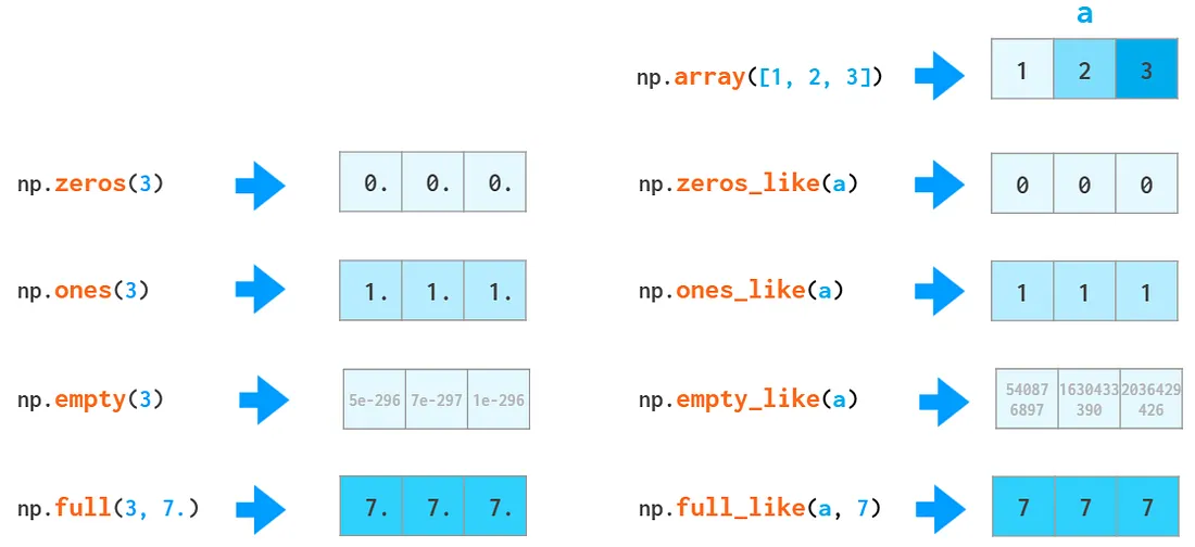
You can create new arrays in a couple different ways. NumPy has shortcuts for the most used types of arrays.
creating a simple (nested) list and turning it into an array with np.array(…) (as we did above)
creating an array filled with zeros with np.zeros
creating an array filled with ones with np.ones
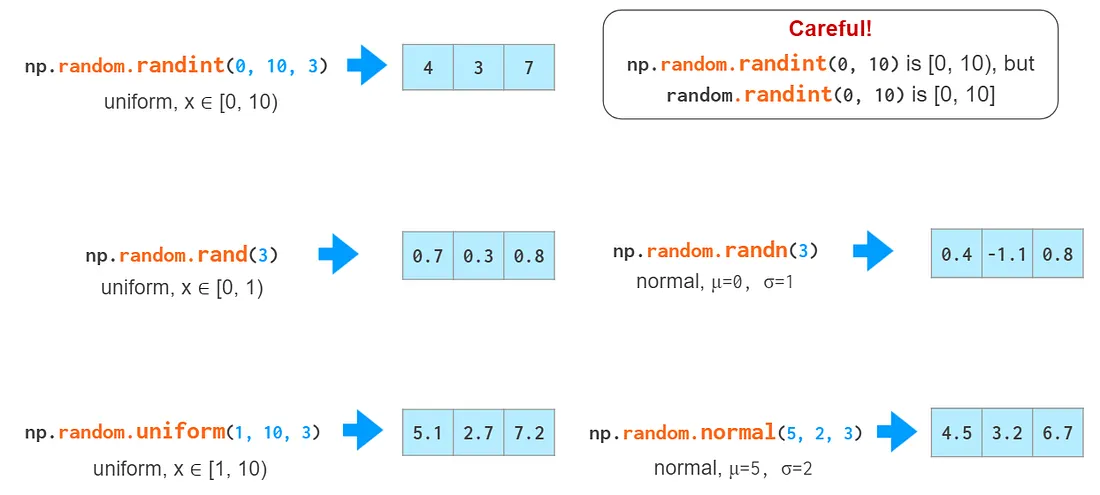
creating an array filled with random values np.random.rand (draws from a uniform distribution)
… many more, like random values drawn from different distributions, triangular matrices, diagonal matrices, etc
[12]:
print("--- Matrix b ---")
print(b)


print("\n--- 3x4 array filled with zeros  ---")
b_zeros = np.zeros((3,4)) # 3x4 array filled with zeros
print(b_zeros)


print("\n--- 3x4 array filled with ones  ---")
b_ones = np.ones((3,4)) # 3x4 array filled with ones
print(b_ones)

print("\n--- 3x4 array filled with random numbers  ---")
b_rand = np.random.rand(3,4) # 3x4 array filled with random numbers
print(b_rand)


# by default most arrays have dtype float64
# but you can change it when you create it!

print("\n--- 3x4 array filled with zeros (default)  ---")
b_zeros = np.zeros((3,4)) # 3x4 array filled with zeros
print(b_zeros)
print(b_zeros.dtype)
print()

print("\n--- 3x4 array filled with zeros (dtype=int)  ---")
b_zeros = np.zeros_like(b, dtype=int) # 3x4 array filled with zeros (integers)
print(b_zeros)
print(b_zeros.dtype)
print()

print("\n--- 3x4 array filled with zeros (dtype=bool)  ---")
b_zeros = np.zeros_like(b, dtype=bool) # 3x4 array filled with zeros (as booleans... so filled with False)
print(b_zeros)
print(b_zeros.dtype)
print()
--- Matrix b ---
[[1 5 2 0]
 [8 3 6 1]
 [1 7 2 9]]

--- 3x4 array filled with zeros  ---
[[0. 0. 0. 0.]
 [0. 0. 0. 0.]
 [0. 0. 0. 0.]]

--- 3x4 array filled with ones  ---
[[1. 1. 1. 1.]
 [1. 1. 1. 1.]
 [1. 1. 1. 1.]]

--- 3x4 array filled with random numbers  ---
[[0.83898056 0.54267576 0.03112879 0.96595569]
 [0.52022488 0.50293211 0.73434727 0.37028894]
 [0.06310305 0.43831281 0.13771197 0.35382173]]

--- 3x4 array filled with zeros (default)  ---
[[0. 0. 0. 0.]
 [0. 0. 0. 0.]
 [0. 0. 0. 0.]]
float64


--- 3x4 array filled with zeros (dtype=int)  ---
[[0 0 0 0]
 [0 0 0 0]
 [0 0 0 0]]
int64


--- 3x4 array filled with zeros (dtype=bool)  ---
[[False False False False]
 [False False False False]
 [False False False False]]
bool
1.6 Basic operations with arrays
They are similar to matricies in maths, so you can do a lot of basic operations with them.
Operations are carried out between corresponding cells.
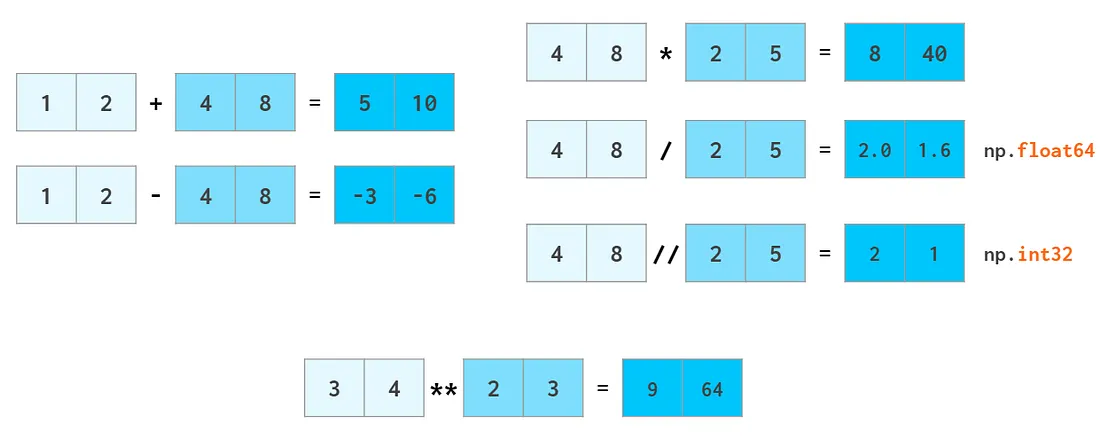
Let’s take for examples the following two arrays, data1 and data2
data1   data2
┌───┐   ┌───┐
│ 1 │   │ 3 │
├───┤   ├───┤
│ 2 │   │ 4 │
└───┘   └───┘
Let’s try and see the results of some basic math operations on them.
[13]:
data1 = np.array([1,2])
data2 = np.array([3,4])

print("(+)", data1 + data2)
print("(-)", data1 - data2)
print("(*)", data1 * data2)
print("(/)", data1 / data2)
(+) [4 6]
(-) [-2 -2]
(*) [3 8]
(/) [0.33333333 0.5       ]
But you can also use single numbers and they will be “promoted to arrays” (aka, broadcasted)
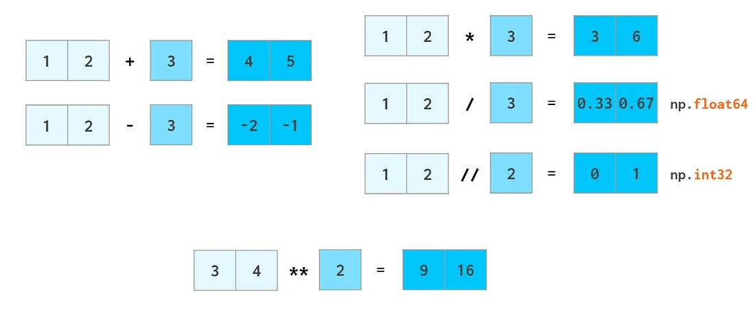
[14]:
print("(+2)", data1 + 2)
print("(-2)", data1 - 2)
print("(*2)", data1 * 2)
print("(/2)", data1 / 2)
(+2) [3 4]
(-2) [-1  0]
(*2) [2 4]
(/2) [0.5 1. ]
1.7 Getting statistics from arrays
Some interesting statistics you can get from arrays are the following:
max value (in general, for each row, for each column)
min value
mean value
standard deviation
…
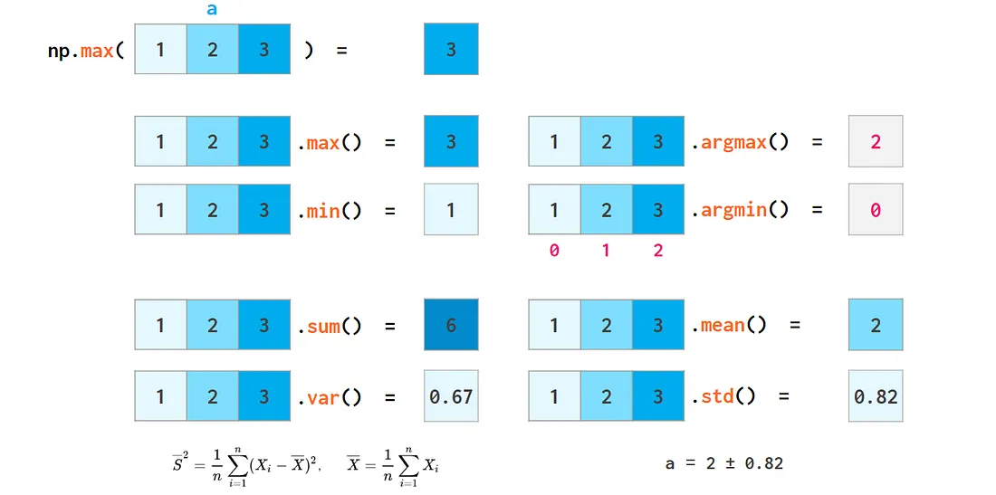
When getting these statistics, you can specify an axis to perform the operation on. For example, on a 2D array:
axis=None(or not giving an axis argument) means collapsing the whole array and to get a single resultaxis=0means collapse the rows (the 0th dimension) to get a result for each columnaxis=1means collapse the columns (the 1st dimension) to get a result for each row
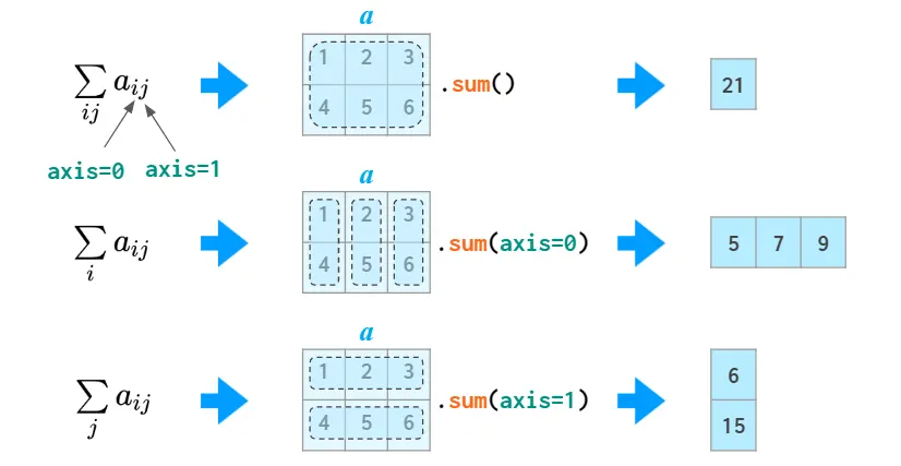
[15]:
print("--- Matrix b ---")
print(b)

print("\n--- max value for the whole array ---")
print(b.max()) # max value for the whole array
print("\n--- max value for each column ---")
print(b.max(axis=0)) # max values for each column
print("\n--- max value for each row ---")
print(b.max(axis=1)) # max values for each row

print("\n\n--- min value for the whole array ---")
print(b.min()) # min value for the whole array
print("\n--- min value for each column ---")
print(b.min(axis=0)) # min values for each column
print("\n--- min value for each row ---")
print(b.min(axis=1)) # min values for each row

print("\n\n--- mean value for the whole array ---")
print(b.mean()) # mean value for the whole array

print("\n\n--- standard deviation for the whole array ---")
print(b.std()) # standard deviation for the whole array
--- Matrix b ---
[[1 5 2 0]
 [8 3 6 1]
 [1 7 2 9]]

--- max value for the whole array ---
9

--- max value for each column ---
[8 7 6 9]

--- max value for each row ---
[5 8 9]


--- min value for the whole array ---
0

--- min value for each column ---
[1 3 2 0]

--- min value for each row ---
[0 1 1]


--- mean value for the whole array ---
3.75


--- standard deviation for the whole array ---
2.9755951785595207
2. Pandas: what and why?
Why pandas?
Handling Tabular Data: It excels at working with tables (rows and columns).
Labeled Data: DataFrames have labeled rows (an Index) and labeled columns, making data access intuitive… no more numerical indexing like in numpy!
Missing Data: It has built-in features to easily manage missing values.
It can be imported as follows:
import pandas as pd
[16]:
import pandas as pd
2.1 What is a DataFrame?
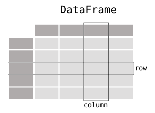
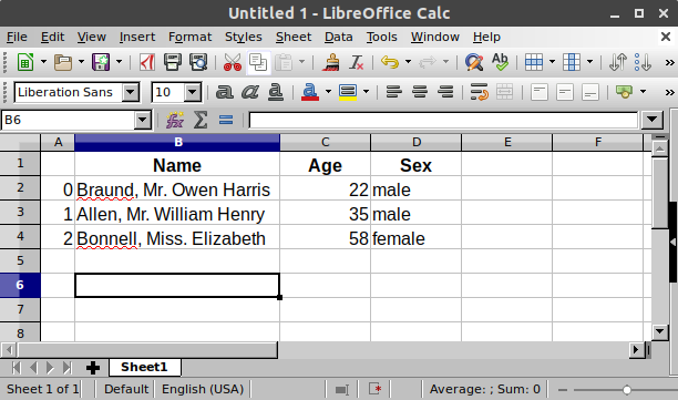
[17]:
df = pd.DataFrame(
    {
        "Name": [
            "Braund, Mr. Owen Harris",
            "Allen, Mr. William Henry",
            "Bonnell, Miss. Elizabeth",
        ],
        "Age": [22, 35, 58],
        "Sex": ["male", "male", "female"],
    }
)
df
[17]:
| Name | Age | Sex | |
|---|---|---|---|
| 0 | Braund, Mr. Owen Harris | 22 | male |
| 1 | Allen, Mr. William Henry | 35 | male |
| 2 | Bonnell, Miss. Elizabeth | 58 | female |
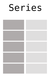
[18]:
# example of the Series "Age"
df["Age"]
[18]:
| Age | |
|---|---|
| 0 | 22 |
| 1 | 35 |
| 2 | 58 |
2.2 Reading and saving data
This is the most practical use of pandas: you can read any kind of tabular data (csv, excel files, json files, …), manipulate them as DataFrame, and then save them back to disk in any format.
The most basic functions are the following:
pd.read_csv(path)read the csv file found atpathand turn it into a DataFrame. Similar functions exist for other types of data (e.g.,pd.read_json,pd.read_excel,pd.read_html,pd.read_sql, …)df.to_csv(path)save the dataframedfat the desiredpathas a csv file. Similar functions exist to save the output as other types of data (e.g.,df.to_json,df.to_excel,df.to_html,df.to_sql, …)
[19]:
# example: read the csv file "sample_data/california_housing_test.csv"
df = pd.read_csv("sample_data/california_housing_test.csv")

display(df)

# example: save it as a json file in the same folder
df.to_json("sample_data/california_housing_test.json")
| longitude | latitude | housing_median_age | total_rooms | total_bedrooms | population | households | median_income | median_house_value | |
|---|---|---|---|---|---|---|---|---|---|
| 0 | -122.05 | 37.37 | 27.0 | 3885.0 | 661.0 | 1537.0 | 606.0 | 6.6085 | 344700.0 |
| 1 | -118.30 | 34.26 | 43.0 | 1510.0 | 310.0 | 809.0 | 277.0 | 3.5990 | 176500.0 |
| 2 | -117.81 | 33.78 | 27.0 | 3589.0 | 507.0 | 1484.0 | 495.0 | 5.7934 | 270500.0 |
| 3 | -118.36 | 33.82 | 28.0 | 67.0 | 15.0 | 49.0 | 11.0 | 6.1359 | 330000.0 |
| 4 | -119.67 | 36.33 | 19.0 | 1241.0 | 244.0 | 850.0 | 237.0 | 2.9375 | 81700.0 |
| ... | ... | ... | ... | ... | ... | ... | ... | ... | ... |
| 2995 | -119.86 | 34.42 | 23.0 | 1450.0 | 642.0 | 1258.0 | 607.0 | 1.1790 | 225000.0 |
| 2996 | -118.14 | 34.06 | 27.0 | 5257.0 | 1082.0 | 3496.0 | 1036.0 | 3.3906 | 237200.0 |
| 2997 | -119.70 | 36.30 | 10.0 | 956.0 | 201.0 | 693.0 | 220.0 | 2.2895 | 62000.0 |
| 2998 | -117.12 | 34.10 | 40.0 | 96.0 | 14.0 | 46.0 | 14.0 | 3.2708 | 162500.0 |
| 2999 | -119.63 | 34.42 | 42.0 | 1765.0 | 263.0 | 753.0 | 260.0 | 8.5608 | 500001.0 |
3000 rows × 9 columns
2.3 Inspecting Data
Once a DataFrame is loaded (from a dictionary, CSV, or any source), the first thing you must do is inspect it to ensure it loaded correctly, check the size, and look at the data types.
The following methods are essential for this inspection:
df.head(): displays the first \(n\) rows of the DataFrame (defaults to \(5\)).df.tail(): displays the last \(n\) rows of the DataFrame (defaults to \(5\)).df.columns: lists the names of all the columns of the DataFrame.df.info(): prints a summary of the DataFrame, including the column names, the number of non-null values, and the data type (\(\mathtt{dtype}\)) for each column.df.shape: returns a tuple representing the dimensions (\(\text{rows} \times \text{columns}\)).df.describe(): generates descriptive statistics (count, mean, standard deviation, min/max) for numerical columns only.
Let’s use the df we loaded from california_housing_test.csv and inspect it:
[20]:
# 1. Look at the top 5 rows
print("--- Head (Top 5 rows) ---")
display(df.head())

# 2. Look at the last 5 rows
print("--- Tail (last 5 rows) ---")
display(df.tail())

# 3. Check all column names
print("--- Columns ---")
display(df.columns)

# 4. Check the overall structure and data types
print("\n--- Info (Data Types and Nulls) ---")
df.info()

# 5. Check the size
print(f"\nDataFrame shape: {df.shape}")

# 6. Get statistics for numerical columns
print("\n--- Descriptive Statistics ---")
display(df.describe())
--- Head (Top 5 rows) ---
| longitude | latitude | housing_median_age | total_rooms | total_bedrooms | population | households | median_income | median_house_value | |
|---|---|---|---|---|---|---|---|---|---|
| 0 | -122.05 | 37.37 | 27.0 | 3885.0 | 661.0 | 1537.0 | 606.0 | 6.6085 | 344700.0 |
| 1 | -118.30 | 34.26 | 43.0 | 1510.0 | 310.0 | 809.0 | 277.0 | 3.5990 | 176500.0 |
| 2 | -117.81 | 33.78 | 27.0 | 3589.0 | 507.0 | 1484.0 | 495.0 | 5.7934 | 270500.0 |
| 3 | -118.36 | 33.82 | 28.0 | 67.0 | 15.0 | 49.0 | 11.0 | 6.1359 | 330000.0 |
| 4 | -119.67 | 36.33 | 19.0 | 1241.0 | 244.0 | 850.0 | 237.0 | 2.9375 | 81700.0 |
--- Tail (last 5 rows) ---
| longitude | latitude | housing_median_age | total_rooms | total_bedrooms | population | households | median_income | median_house_value | |
|---|---|---|---|---|---|---|---|---|---|
| 2995 | -119.86 | 34.42 | 23.0 | 1450.0 | 642.0 | 1258.0 | 607.0 | 1.1790 | 225000.0 |
| 2996 | -118.14 | 34.06 | 27.0 | 5257.0 | 1082.0 | 3496.0 | 1036.0 | 3.3906 | 237200.0 |
| 2997 | -119.70 | 36.30 | 10.0 | 956.0 | 201.0 | 693.0 | 220.0 | 2.2895 | 62000.0 |
| 2998 | -117.12 | 34.10 | 40.0 | 96.0 | 14.0 | 46.0 | 14.0 | 3.2708 | 162500.0 |
| 2999 | -119.63 | 34.42 | 42.0 | 1765.0 | 263.0 | 753.0 | 260.0 | 8.5608 | 500001.0 |
--- Columns ---
Index(['longitude', 'latitude', 'housing_median_age', 'total_rooms',
       'total_bedrooms', 'population', 'households', 'median_income',
       'median_house_value'],
      dtype='object')
--- Info (Data Types and Nulls) ---
<class 'pandas.core.frame.DataFrame'>
RangeIndex: 3000 entries, 0 to 2999
Data columns (total 9 columns):
 #   Column              Non-Null Count  Dtype
---  ------              --------------  -----
 0   longitude           3000 non-null   float64
 1   latitude            3000 non-null   float64
 2   housing_median_age  3000 non-null   float64
 3   total_rooms         3000 non-null   float64
 4   total_bedrooms      3000 non-null   float64
 5   population          3000 non-null   float64
 6   households          3000 non-null   float64
 7   median_income       3000 non-null   float64
 8   median_house_value  3000 non-null   float64
dtypes: float64(9)
memory usage: 211.1 KB

DataFrame shape: (3000, 9)

--- Descriptive Statistics ---
| longitude | latitude | housing_median_age | total_rooms | total_bedrooms | population | households | median_income | median_house_value | |
|---|---|---|---|---|---|---|---|---|---|
| count | 3000.000000 | 3000.00000 | 3000.000000 | 3000.000000 | 3000.000000 | 3000.000000 | 3000.00000 | 3000.000000 | 3000.00000 |
| mean | -119.589200 | 35.63539 | 28.845333 | 2599.578667 | 529.950667 | 1402.798667 | 489.91200 | 3.807272 | 205846.27500 |
| std | 1.994936 | 2.12967 | 12.555396 | 2155.593332 | 415.654368 | 1030.543012 | 365.42271 | 1.854512 | 113119.68747 |
| min | -124.180000 | 32.56000 | 1.000000 | 6.000000 | 2.000000 | 5.000000 | 2.00000 | 0.499900 | 22500.00000 |
| 25% | -121.810000 | 33.93000 | 18.000000 | 1401.000000 | 291.000000 | 780.000000 | 273.00000 | 2.544000 | 121200.00000 |
| 50% | -118.485000 | 34.27000 | 29.000000 | 2106.000000 | 437.000000 | 1155.000000 | 409.50000 | 3.487150 | 177650.00000 |
| 75% | -118.020000 | 37.69000 | 37.000000 | 3129.000000 | 636.000000 | 1742.750000 | 597.25000 | 4.656475 | 263975.00000 |
| max | -114.490000 | 41.92000 | 52.000000 | 30450.000000 | 5419.000000 | 11935.000000 | 4930.00000 | 15.000100 | 500001.00000 |
2.4 Accessing data
After inspection, the next step is accessing specific parts of the data.
2.4.1 Accessing columns
To select one or more columns, you use their name in square brackets just like accessing items in a Python dictionary.
df["col_name"], selecting a single column returns a Pandas Series.df[["col_name1", "col_name2"]], selecting a list of columns returns a new DataFrame.
[21]:
# Select a single column (output is a Series)
print("--- 1. Select the 'housing_median_age' column (Series) ---")
display(df['housing_median_age'].head(3))

# Select multiple columns (output is a new DataFrame)
print("\n--- 2. Select 'total_rooms' and 'median_income' (DataFrame) ---")
display(df[['total_rooms', 'median_income']].head(3))
--- 1. Select the 'housing_median_age' column (Series) ---
| housing_median_age | |
|---|---|
| 0 | 27.0 |
| 1 | 43.0 |
| 2 | 27.0 |
--- 2. Select 'total_rooms' and 'median_income' (DataFrame) ---
| total_rooms | median_income | |
|---|---|---|
| 0 | 3885.0 | 6.6085 |
| 1 | 1510.0 | 3.5990 |
| 2 | 3589.0 | 5.7934 |
2.4.2 Accessing rows
To select one or more rows, you can use their index and the accessor ``.loc[]``
df.loc[0], selecting a single row returns a Pandas Series.df.loc[[0,3]], selecting a list of rows returns a new DataFrame.
Or, you can use their position and the accessor ``.iloc[]``
loc and iloc may seem similar (they work the same in these basic examples). But in more complex cases they behave different (e.g., if your index contains strings or is shuffled after working on it, you will need iloc to select the 0th row).
[22]:
# Select a single row (output is a Series)
print("--- 1. Select row 0 (Series) ---")
display(df.loc[0])

# Select multiple rows (output is a new DataFrame)
print("\n--- 2. Select row 0, 3, and 5 (DataFrame) ---")
display(df.loc[[0,3,5]])
--- 1. Select row 0 (Series) ---
| 0 | |
|---|---|
| longitude | -122.0500 |
| latitude | 37.3700 |
| housing_median_age | 27.0000 |
| total_rooms | 3885.0000 |
| total_bedrooms | 661.0000 |
| population | 1537.0000 |
| households | 606.0000 |
| median_income | 6.6085 |
| median_house_value | 344700.0000 |
--- 2. Select row 0, 3, and 5 (DataFrame) ---
| longitude | latitude | housing_median_age | total_rooms | total_bedrooms | population | households | median_income | median_house_value | |
|---|---|---|---|---|---|---|---|---|---|
| 0 | -122.05 | 37.37 | 27.0 | 3885.0 | 661.0 | 1537.0 | 606.0 | 6.6085 | 344700.0 |
| 3 | -118.36 | 33.82 | 28.0 | 67.0 | 15.0 | 49.0 | 11.0 | 6.1359 | 330000.0 |
| 5 | -119.56 | 36.51 | 37.0 | 1018.0 | 213.0 | 663.0 | 204.0 | 1.6635 | 67000.0 |
2.4.3 Accessing values
loc and iloc can be used to specify columns too using the format:df.loc[row_labels(s), column_label(s)].Remember: loc works with labels (index and column names) while iloc works with positions (row number and column number).
df.loc[0, "col_name"], selecting a single row and column, returns a value.df.loc[0:3, ["col_name1", "col_name2"]], selecting a list of rows and columns returns a new DataFrame.
Like in numpy arrays, you can use “:” to signify “all values” if you want to keep all columns/all rows.
[23]:
# Select all columns (using :) for rows 0 through 4 (inclusive of 4)
print("--- 1. Rows 0 through 4, All Columns (using labels) ---")
display(df.loc[0:4, :])

# Select rows 1 and 3, and only the 'latitude' and 'longitude' columns
print("\n--- 2. Specific Rows and Specific Columns (using labels) ---")
# Note: Since our index defaults to numbers, we can use numbers as labels here.
display(df.loc[[1, 3], ['latitude', 'longitude']])
--- 1. Rows 0 through 4, All Columns (using labels) ---
| longitude | latitude | housing_median_age | total_rooms | total_bedrooms | population | households | median_income | median_house_value | |
|---|---|---|---|---|---|---|---|---|---|
| 0 | -122.05 | 37.37 | 27.0 | 3885.0 | 661.0 | 1537.0 | 606.0 | 6.6085 | 344700.0 |
| 1 | -118.30 | 34.26 | 43.0 | 1510.0 | 310.0 | 809.0 | 277.0 | 3.5990 | 176500.0 |
| 2 | -117.81 | 33.78 | 27.0 | 3589.0 | 507.0 | 1484.0 | 495.0 | 5.7934 | 270500.0 |
| 3 | -118.36 | 33.82 | 28.0 | 67.0 | 15.0 | 49.0 | 11.0 | 6.1359 | 330000.0 |
| 4 | -119.67 | 36.33 | 19.0 | 1241.0 | 244.0 | 850.0 | 237.0 | 2.9375 | 81700.0 |
--- 2. Specific Rows and Specific Columns (using labels) ---
| latitude | longitude | |
|---|---|---|
| 1 | 34.26 | -118.30 |
| 3 | 33.82 | -118.36 |
[24]:
# Select rows from position 0 up to (but not including) position 5
# and columns from position 1 up to (but not including) position 3.
print("--- Rows 0-4, Columns 1-2 (strictly by position) ---")
# Columns 1 and 2 correspond to 'latitude' and 'longitude'
display(df.iloc[0:5, 1:3])

# Select row at position 2 and column at position 5 (single element)
print("\n--- Single element: Row position 2, Column position 5 ---")
# Position 5 is 'households'
print(df.iloc[2, 5])
--- Rows 0-4, Columns 1-2 (strictly by position) ---
| latitude | housing_median_age | |
|---|---|---|
| 0 | 37.37 | 27.0 |
| 1 | 34.26 | 43.0 |
| 2 | 33.78 | 27.0 |
| 3 | 33.82 | 28.0 |
| 4 | 36.33 | 19.0 |
--- Single element: Row position 2, Column position 5 ---
1484.0
2.5 Filtering data
Filtering allows you to select only the rows that meet a specific set of conditions. This technique uses Boolean Masks (a core concept from NumPy) where we create a Series of True/False values, and then pass that Series back into the DataFrame to select only the rows where the mask is True.
To filter with a single condition, you state the condition inside the square brackets of the DataFrame:
df[condition]When you need to use more than one condition, you must wrap each condition in parentheses and use the NumPy-style logical operators (and is
&, or is|)
[25]:
# 1. Create a Series of True/False values (the Boolean Mask)
# We are checking which rows have an 'housing_median_age' less than 20
bool_mask = df['housing_median_age'] < 20
print("--- Boolean Mask (True/False Series) ---")
display(bool_mask.head())

# 2. Use the mask to filter the DataFrame
# This returns a new DataFrame containing only the rows where the mask was True.
masked_df = df[bool_mask]

print(f"\n--- Filtered DataFrame (showing the first 5 rows) ---")
print(f"Original shape: {df.shape}")
print(f"Filtered shape: {masked_df.shape}")
display(masked_df.head())
--- Boolean Mask (True/False Series) ---
| housing_median_age | |
|---|---|
| 0 | False |
| 1 | False |
| 2 | False |
| 3 | False |
| 4 | True |
--- Filtered DataFrame (showing the first 5 rows) ---
Original shape: (3000, 9)
Filtered shape: (830, 9)
| longitude | latitude | housing_median_age | total_rooms | total_bedrooms | population | households | median_income | median_house_value | |
|---|---|---|---|---|---|---|---|---|---|
| 4 | -119.67 | 36.33 | 19.0 | 1241.0 | 244.0 | 850.0 | 237.0 | 2.9375 | 81700.0 |
| 7 | -120.65 | 35.48 | 19.0 | 2310.0 | 471.0 | 1341.0 | 441.0 | 3.2250 | 166900.0 |
| 8 | -122.84 | 38.40 | 15.0 | 3080.0 | 617.0 | 1446.0 | 599.0 | 3.6696 | 194400.0 |
| 13 | -117.03 | 32.97 | 16.0 | 3936.0 | 694.0 | 1935.0 | 659.0 | 4.5625 | 231200.0 |
| 16 | -120.81 | 37.53 | 15.0 | 570.0 | 123.0 | 189.0 | 107.0 | 1.8750 | 181300.0 |
[26]:
# Select rows where:
# 1. The housing_median_age is less than 20
# AND
# 2. The median_house_value is greater than 300000
two_conditions_df = df[
    (df['housing_median_age'] < 20) &
    (df['median_house_value'] > 300000)
]

print(f"Filtered shape: {two_conditions_df.shape}")
display(two_conditions_df.head())
Filtered shape: (115, 9)
| longitude | latitude | housing_median_age | total_rooms | total_bedrooms | population | households | median_income | median_house_value | |
|---|---|---|---|---|---|---|---|---|---|
| 28 | -118.45 | 34.07 | 19.0 | 4845.0 | 1609.0 | 3751.0 | 1539.0 | 1.5830 | 350000.0 |
| 78 | -118.75 | 34.17 | 18.0 | 6217.0 | 858.0 | 2703.0 | 834.0 | 6.8075 | 325900.0 |
| 118 | -117.18 | 33.02 | 15.0 | 3540.0 | 453.0 | 1364.0 | 425.0 | 13.6623 | 500001.0 |
| 124 | -117.81 | 33.84 | 17.0 | 4343.0 | 515.0 | 1605.0 | 484.0 | 10.5981 | 460100.0 |
| 152 | -117.91 | 33.94 | 15.0 | 5799.0 | 842.0 | 2314.0 | 787.0 | 6.3433 | 350500.0 |
2.6 Adding and Modifying Columns
One of the most common tasks in data analysis is creating new features or columns based on transformations of existing data. Pandas makes this very easy using vectorized operations.
You can create a new column by simply using the name of the new column on the left side, and a calculation on the right side. This uses vectorization, which is fast because it operates on entire columns at once (leveraging NumPy’s efficiency).
For example, we can calculate the average number of rooms per household:
[27]:
# Create a new column 'rooms_per_household'
df['rooms_per_household'] = df['total_rooms'] / df['households']

# Display the new column alongside the columns used to create it
print("--- New Column Created by Vectorized Operation ---")
display(df[['total_rooms', 'households', 'rooms_per_household']].head())
--- New Column Created by Vectorized Operation ---
| total_rooms | households | rooms_per_household | |
|---|---|---|---|
| 0 | 3885.0 | 606.0 | 6.410891 |
| 1 | 1510.0 | 277.0 | 5.451264 |
| 2 | 3589.0 | 495.0 | 7.250505 |
| 3 | 67.0 | 11.0 | 6.090909 |
| 4 | 1241.0 | 237.0 | 5.236287 |
[28]:
# Create a new column 'people_per_household', based on 'population' and 'households'
df['people_per_household'] = df['population'] / df['households']

# Display the new column alongside the columns used to create it
print("--- New Column Created by Vectorized Operation ---")
display(df[['population', 'households', 'people_per_household']].head())
--- New Column Created by Vectorized Operation ---
| population | households | people_per_household | |
|---|---|---|---|
| 0 | 1537.0 | 606.0 | 2.536304 |
| 1 | 809.0 | 277.0 | 2.920578 |
| 2 | 1484.0 | 495.0 | 2.997980 |
| 3 | 49.0 | 11.0 | 4.454545 |
| 4 | 850.0 | 237.0 | 3.586498 |
2.7 Basic Aggregation and Statistics
One of the main reasons we use Pandas is to get quick summaries and statistics from our data. Unlike NumPy, Pandas uses methods that are specific to the labeled Series (columns).
You can easily get statistical summaries for a single column, or for the entire DataFrame.
Applying a statistical method directly to a DataFrame will run that calculation on every numerical column, returning a Series of results.
[29]:
# Calculate the mean (average) of every numerical column in the DataFrame
print("--- Mean of all numerical columns ---")
display(df.mean())

# Calculate the maximum value found in every numerical column
print("\n--- Maximum value of all numerical columns ---")
display(df.max())
--- Mean of all numerical columns ---
| 0 | |
|---|---|
| longitude | -119.589200 |
| latitude | 35.635390 |
| housing_median_age | 28.845333 |
| total_rooms | 2599.578667 |
| total_bedrooms | 529.950667 |
| population | 1402.798667 |
| households | 489.912000 |
| median_income | 3.807272 |
| median_house_value | 205846.275000 |
| rooms_per_household | 5.406560 |
| people_per_household | 3.035270 |
--- Maximum value of all numerical columns ---
| 0 | |
|---|---|
| longitude | -114.490000 |
| latitude | 41.920000 |
| housing_median_age | 52.000000 |
| total_rooms | 30450.000000 |
| total_bedrooms | 5419.000000 |
| population | 11935.000000 |
| households | 4930.000000 |
| median_income | 15.000100 |
| median_house_value | 500001.000000 |
| rooms_per_household | 62.422222 |
| people_per_household | 230.172414 |
To focus your analysis, you often want to get statistics for a specific column. Since each column is a Pandas Series, you apply the method directly to the selected Series.
[30]:
# Select the 'median_income' column and calculate its standard deviation (std)
print("--- Standard Deviation of 'median_income' ---")
print(df['median_income'].std())

# Select the 'population' column and calculate its sum
print("\n--- Total 'population' ---")
print(df['population'].sum())

# Calculate how many unique values are in the 'ocean_proximity' column
print("\n--- Unique Values in 'housing_median_age' ---")
print(df['housing_median_age'].nunique())

# Get a count of each unique value (very common for categorical data)
print("\n--- Count of each 'housing_median_age' category ---")
display(df['housing_median_age'].value_counts())
--- Standard Deviation of 'median_income' ---
1.854511729691481

--- Total 'population' ---
4208396.0

--- Unique Values in 'housing_median_age' ---
52

--- Count of each 'housing_median_age' category ---
| count | |
|---|---|
| housing_median_age | |
| 52.0 | 173 |
| 35.0 | 118 |
| 36.0 | 115 |
| 16.0 | 107 |
| 34.0 | 102 |
| 17.0 | 100 |
| 32.0 | 91 |
| 37.0 | 88 |
| 26.0 | 88 |
| 25.0 | 86 |
| 33.0 | 85 |
| 15.0 | 77 |
| 30.0 | 76 |
| 19.0 | 76 |
| 18.0 | 76 |
| 24.0 | 75 |
| 29.0 | 75 |
| 27.0 | 74 |
| 38.0 | 64 |
| 20.0 | 63 |
| 21.0 | 61 |
| 22.0 | 60 |
| 28.0 | 58 |
| 31.0 | 57 |
| 14.0 | 57 |
| 43.0 | 56 |
| 41.0 | 56 |
| 39.0 | 55 |
| 23.0 | 53 |
| 45.0 | 51 |
| 44.0 | 51 |
| 42.0 | 51 |
| 40.0 | 43 |
| 13.0 | 41 |
| 46.0 | 41 |
| 12.0 | 41 |
| 11.0 | 41 |
| 5.0 | 39 |
| 48.0 | 34 |
| 10.0 | 30 |
| 4.0 | 28 |
| 9.0 | 27 |
| 8.0 | 25 |
| 6.0 | 25 |
| 47.0 | 22 |
| 49.0 | 21 |
| 7.0 | 20 |
| 50.0 | 16 |
| 3.0 | 12 |
| 51.0 | 11 |
| 2.0 | 6 |
| 1.0 | 2 |